Northumbria nursing lecturer named Nurse Educator of the Year at prestigious national awards
A Northumbria University academic has been named Nurse Educator of the Year at the British…


A Northumbria University academic has been named Nurse Educator of the Year at the British…

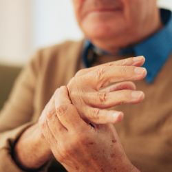
Northumbria University is spearheading a major international research initiative that explores…
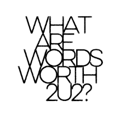
Programme Northumbria is delighted to present What Are Words Worth 2U2?, an interdisciplinary,…

Northumbria University’s annual REVEAL degree shows spotlight the exceptional work of graduating…

Northumbria University is set to throw open its doors to the public this May as part of The…

Northumbria University's Newcastle Business School has secured reaccreditation with the Small…

Three academics from Northumbria University have been shortlisted for the Graduate Futures…
Two Northumbria University researchers are among 55 early career scientists across the UK to…

Ellison Building (ELA 101)
-
The Great Hall
-

